How to graph the function y=sin x? First, let's look at the sine graph on the interval.
We take a single segment 2 cells long in the notebook. On the Oy axis we mark one.
For convenience, we round the number π/2 to 1.5 (and not to 1.6, as required by the rounding rules). In this case, a segment of length π/2 corresponds to 3 cells.
On the Ox axis we mark not single segments, but segments of length π/2 (every 3 cells). Accordingly, a segment of length π corresponds to 6 cells, and a segment of length π/6 corresponds to 1 cell.
With this choice of a unit segment, the graph depicted on a sheet of notebook in a box corresponds as much as possible to the graph of the function y=sin x.
Let's make a table of sine values on the interval:
We mark the resulting points on the coordinate plane:

Since y=sin x is an odd function, the sine graph is symmetrical with respect to the origin - point O(0;0). Taking this fact into account, let’s continue plotting the graph to the left, then the points -π:

The function y=sin x is periodic with period T=2π. Therefore, the graph of a function taken on the interval [-π;π] is repeated an infinite number of times to the right and to the left.
, Competition "Presentation for the lesson"
Presentation for the lesson


 Back Forward
Attention! Slide previews are for informational purposes only and may not represent all of the presentation's features. If you are interested in this work, please download the full version.
Iron rusts without finding any use,
standing water rots or freezes in the cold,
and a person’s mind, not finding any use for itself, languishes.
Leonardo da Vinci
Technologies used: problem-based learning, critical thinking, communicative communication.
Goals:
- Development of cognitive interest in learning.
- Studying the properties of the function y = sin x.
- Formation of practical skills in constructing a graph of the function y = sin x based on the studied theoretical material.
Tasks:
1. Use the existing potential of knowledge about the properties of the function y = sin x in specific situations.
2. Apply conscious establishment of connections between analytical and geometric models of the function y = sin x.
Develop initiative, a certain willingness and interest in finding a solution; the ability to make decisions, not stop there, and defend your point of view.
To foster in students cognitive activity, a sense of responsibility, respect for each other, mutual understanding, mutual support, and self-confidence; culture of communication.
Lesson progress
Stage 1. Updating basic knowledge, motivating learning new material
"Entering the lesson."
There are 3 statements written on the board:
- The trigonometric equation sin t = a always has solutions.
- The graph of an odd function can be constructed using a symmetry transformation about the Oy axis.
- A trigonometric function can be graphed using one principal half-wave.
Students discuss in pairs: are the statements true? (1 minute). The results of the initial discussion (yes, no) are then entered into the table in the "Before" column.
The teacher sets the goals and objectives of the lesson.
2. Updating knowledge (frontally on a model of a trigonometric circle).
We have already become acquainted with the function s = sin t.
1) What values can the variable t take. What is the scope of this function?
2) In what interval are the values of the expression sin t contained? Find the largest and smallest values of the function s = sin t.
3) Solve the equation sin t = 0.
4) What happens to the ordinate of a point as it moves along the first quarter? (the ordinate increases). What happens to the ordinate of a point as it moves along the second quarter? (the ordinate gradually decreases). How does this relate to the monotonicity of the function? (the function s = sin t increases on the segment and decreases on the segment ).
5) Let’s write the function s = sin t in the form y = sin x that is familiar to us (we will construct it in the usual xOy coordinate system) and compile a table of the values of this function.
| X | 0 | ||||||
| at | 0 | 1 | 0 |
Stage 2. Perception, comprehension, primary consolidation, involuntary memorization
Stage 4. Primary systematization of knowledge and methods of activity, their transfer and application in new situations
6. No. 10.18 (b,c)
Stage 5. Final control, correction, assessment and self-assessment
7. Return to the statements (beginning of the lesson), discuss using the properties of the trigonometric function y = sin x, and fill in the “After” column in the table.
8. D/z: clause 10, No. 10.7(a), 10.8(b), 10.11(b), 10.16(a)
Centered at a point A.
α
- angle expressed in radians.
Definition
Sine (sin α) is a trigonometric function depending on the angle α between the hypotenuse and the leg of a right triangle, equal to the ratio of the length of the opposite leg |BC| to the length of the hypotenuse |AC|.
Cosine (cos α) is a trigonometric function depending on the angle α between the hypotenuse and the leg of a right triangle, equal to the ratio of the length of the adjacent leg |AB| to the length of the hypotenuse |AC|.
Accepted notations
;
;
.
;
;
.
Graph of the sine function, y = sin x
Graph of the cosine function, y = cos x

Properties of sine and cosine
Periodicity
Functions y = sin x and y = cos x periodic with period 2π.
Parity
The sine function is odd. The cosine function is even.
Domain of definition and values, extrema, increase, decrease
The sine and cosine functions are continuous in their domain of definition, that is, for all x (see proof of continuity). Their main properties are presented in the table (n - integer).
| y = sin x | y = cos x | |
| Scope and continuity | - ∞ < x < + ∞ | - ∞ < x < + ∞ |
| Range of values | -1 ≤ y ≤ 1 | -1 ≤ y ≤ 1 |
| Increasing | ||
| Descending | ||
| Maxima, y = 1 | ||
| Minima, y = - 1 | ||
| Zeros, y = 0 | ||
| Intercept points with the ordinate axis, x = 0 | y = 0 | y = 1 |
Basic formulas
Sum of squares of sine and cosine
Formulas for sine and cosine from sum and difference
;
;
Formulas for the product of sines and cosines
Sum and difference formulas
Expressing sine through cosine
;
;
;
.
Expressing cosine through sine
;
;
;
.
Expression through tangent
; .
When , we have:
;
.
At :
;
.
Table of sines and cosines, tangents and cotangents
This table shows the values of sines and cosines for certain values of the argument. 
Expressions through complex variables
;
Euler's formula
Expressions through hyperbolic functions
;
;
Derivatives
; . Deriving formulas > > >
Derivatives of nth order:
{ -∞ <
x < +∞ }
Secant, cosecant
Inverse functions
The inverse functions of sine and cosine are arcsine and arccosine, respectively.
Arcsine, arcsin
Arccosine, arccos
Used literature:
I.N. Bronstein, K.A. Semendyaev, Handbook of mathematics for engineers and college students, “Lan”, 2009.
Functiony = sinx
The graph of the function is a sinusoid.
The complete non-repeating portion of a sine wave is called a sine wave.
Half a sine wave is called a half sine wave (or arc).
Function Propertiesy =
sinx:
3) This is an odd function. 4) This is a continuous function.
6) On the segment [-π/2; π/2] function increases on the interval [π/2; 3π/2] – decreases. 7) On intervals the function takes positive values. 8) Intervals of increasing function: [-π/2 + 2πn; π/2 + 2πn]. 9) Minimum points of the function: -π/2 + 2πn. |
To graph a function y= sin x It is convenient to use the following scales:
On a sheet of paper with a square, we take the length of two squares as a unit of segment.
On axis x Let's measure the length π. At the same time, for convenience, we present 3.14 in the form of 3 - that is, without a fraction. Then on a sheet of paper in a cell π will be 6 cells (three times 2 cells). And each cell will receive its own natural name (from the first to the sixth): π/6, π/3, π/2, 2π/3, 5π/6, π. These are the meanings x.
On the y-axis we mark 1, which includes two cells.
Let's create a table of function values using our values x:
√3 | √3 |
Next, let's create a schedule. The result is a half-wave, the highest point of which is (π/2; 1). This is the graph of the function y= sin x on the segment. Let's add a symmetrical half-wave to the constructed graph (symmetrical relative to the origin, that is, on the segment -π). The crest of this half-wave is under the x-axis with coordinates (-1; -1). The result will be a wave. This is the graph of the function y= sin x on the segment [-π; π].
You can continue the wave by constructing it on the segment [π; 3π], [π; 5π], [π; 7π], etc. On all these segments, the graph of the function will look the same as on the segment [-π; π]. You will get a continuous wavy line with identical waves.
Functiony = cosx.
The graph of a function is a sine wave (sometimes called a cosine wave).

Function Propertiesy = cosx:
1) The domain of definition of a function is the set of real numbers. 2) The range of function values is the segment [–1; 1] 3) This is an even function. 4) This is a continuous function. 5) Coordinates of the intersection points of the graph: 6) On the segment the function decreases, on the segment [π; 2π] – increases. 7) On intervals [-π/2 + 2πn; π/2 + 2πn] function takes positive values. 8) Increasing intervals: [-π + 2πn; 2πn]. 9) Minimum points of the function: π + 2πn. 10) The function is limited from above and below. The smallest value of the function is –1, 11) This is a periodic function with a period of 2π (T = 2π) |
Functiony = mf(x).
Let's take the previous function y=cos x. As you already know, its graph is a sine wave. If we multiply the cosine of this function by a certain number m, then the wave will expand from the axis x(or will shrink, depending on the value of m).
This new wave will be the graph of the function y = mf(x), where m is any real number.
Thus, the function y = mf(x) is the familiar function y = f(x) multiplied by m.
Ifm< 1, то синусоида сжимается к оси x by the coefficientm. Ifm > 1, then the sinusoid is stretched from the axisx by the coefficientm.
When performing stretching or compression, you can first plot only one half-wave of a sine wave, and then complete the entire graph.
Functiony = f(kx).
If the function y =mf(x) leads to stretching of the sinusoid from the axis x or compression towards the axis x, then the function y = f(kx) leads to stretching from the axis y or compression towards the axis y.
Moreover, k is any real number.
At 0< k< 1 синусоида растягивается от оси y by the coefficientk. Ifk > 1, then the sinusoid is compressed towards the axisy by the coefficientk.
When drawing up a graph of this function, you can first build one half-wave of a sine wave, and then use it to complete the entire graph.
Functiony = tgx.
Function graph y= tg x is a tangent.
It is enough to construct part of the graph in the interval from 0 to π/2, and then you can symmetrically continue it in the interval from 0 to 3π/2.

Function Propertiesy = tgx:
Functiony = ctgx
Function graph y=ctg x is also a tangentoid (it is sometimes called a cotangentoid).

Function Propertiesy = ctgx:
We found out that the behavior of trigonometric functions, and the functions y = sin x in particular, on the entire number line (or for all values of the argument X) is completely determined by its behavior in the interval 0 < X < π / 2 .
Therefore, first of all, we will plot the function y = sin x exactly in this interval.
Let's make the following table of values of our function;
By marking the corresponding points on the coordinate plane and connecting them with a smooth line, we obtain the curve shown in the figure

The resulting curve could also be constructed geometrically, without compiling a table of function values y = sin x .

1. Divide the first quarter of a circle of radius 1 into 8 equal parts. The ordinates of the dividing points of the circle are the sines of the corresponding angles.
2.The first quarter of the circle corresponds to angles from 0 to π / 2 . Therefore, on the axis X Let's take a segment and divide it into 8 equal parts.
3. Let's draw straight lines parallel to the axes X, and from the division points we construct perpendiculars until they intersect with horizontal lines.
4. Connect the intersection points with a smooth line.
Now let's look at the interval π /
2
<
X <
π
.
Each argument value X from this interval can be represented as
x = π / 2 + φ
Where 0 < φ < π / 2 . According to reduction formulas
sin ( π / 2 + φ ) = cos φ = sin ( π / 2 - φ ).
Axis points X with abscissas π / 2 + φ And π / 2 - φ symmetrical to each other about the axis point X with abscissa π / 2 , and the sines at these points are the same. This allows us to obtain a graph of the function y = sin x in the interval [ π / 2 , π ] by simply symmetrically displaying the graph of this function in the interval relative to the straight line X = π / 2 .

Now using the property odd parity function y = sin x,
sin(- X) = - sin X,
it is easy to plot this function in the interval [- π , 0].

The function y = sin x is periodic with a period of 2π ;. Therefore, to construct the entire graph of this function, it is enough to continue the curve shown in the figure to the left and right periodically with a period 2π .
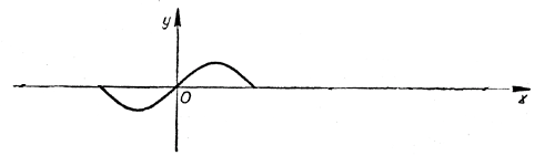
The resulting curve is called sinusoid . This is the graph of the function y = sin x.

The figure illustrates well all the properties of the function y = sin x , which we have previously proven. Let us recall these properties.
1) Function y = sin x defined for all values X , so its domain is the set of all real numbers.
2) Function y = sin x limited. All the values it accepts are between -1 and 1, including these two numbers. Consequently, the range of variation of this function is determined by the inequality -1 < at < 1. When X = π / 2 + 2k π the function takes the largest values equal to 1, and for x = - π / 2 + 2k π - the smallest values equal to - 1.
3) Function y = sin x is odd (the sine wave is symmetrical about the origin).
4) Function y = sin x periodic with period 2 π .
5) In 2n intervals π < x < π + 2n π (n is any integer) it is positive, and in intervals π + 2k π < X < 2π + 2k π (k is any integer) it is negative. At x = k π the function goes to zero. Therefore, these values of the argument x (0; ± π ; ±2 π ; ...) are called function zeros y = sin x
6) At intervals - π / 2 + 2n π < X < π / 2 + 2n π function y = sin x increases monotonically, and in intervals π / 2 + 2k π < X < 3π / 2 + 2k π it decreases monotonically.
You should pay special attention to the behavior of the function y = sin x near the point X = 0 .
For example, sin 0.012 ≈ 0.012; sin(-0.05) ≈ -0,05;
sin 2° = sin π 2 / 180 = sin π / 90 ≈ 0,03 ≈ 0,03.
At the same time, it should be noted that for any values of x
| sin x| < | x | . (1)
Indeed, let the radius of the circle shown in the figure be equal to 1,
a /
AOB = X.

Then sin x= AC. But AC< АВ, а АВ, в свою очередь, меньше длины дуги АВ, на которую опирается угол X. The length of this arc is obviously equal to X, since the radius of the circle is 1. So, at 0< X < π / 2
sin x< х.
Hence, due to the oddness of the function y = sin x it is easy to show that when - π / 2 < X < 0
| sin x| < | x | .
Finally, when x = 0
| sin x | = | x |.
Thus, for | X | < π / 2 inequality (1) has been proven. In fact, this inequality is also true for | x | > π / 2 due to the fact that | sin X | < 1, a π / 2 > 1
Exercises

1.According to the graph of the function y = sin x determine: a) sin 2; b) sin 4; c) sin (-3).
2.According to the graph of the function y = sin x
determine which number from the interval
[ - π /
2 ,
π /
2
] has a sine equal to: a) 0.6; b) -0.8.
3. According to the graph of the function y = sin x
determine which numbers have a sine,
equal to 1/2.
4. Find approximately (without using tables): a) sin 1°; b) sin 0.03;
c) sin (-0.015); d) sin (-2°30").